andersswanson.dev

Want to query graph-shaped relationships in Oracle AI Database from plain JDBC? You can do exactly that with built-in graph capabilities.

In this article, we’ll walk through a sample that shows how to use property graphs in Oracle AI Database, building graph queries over standard relational tables with the GRAPH_TABLE operator.

If you want to skip straight to the code, start here: jdbc-property-graph source code

What we’ll cover

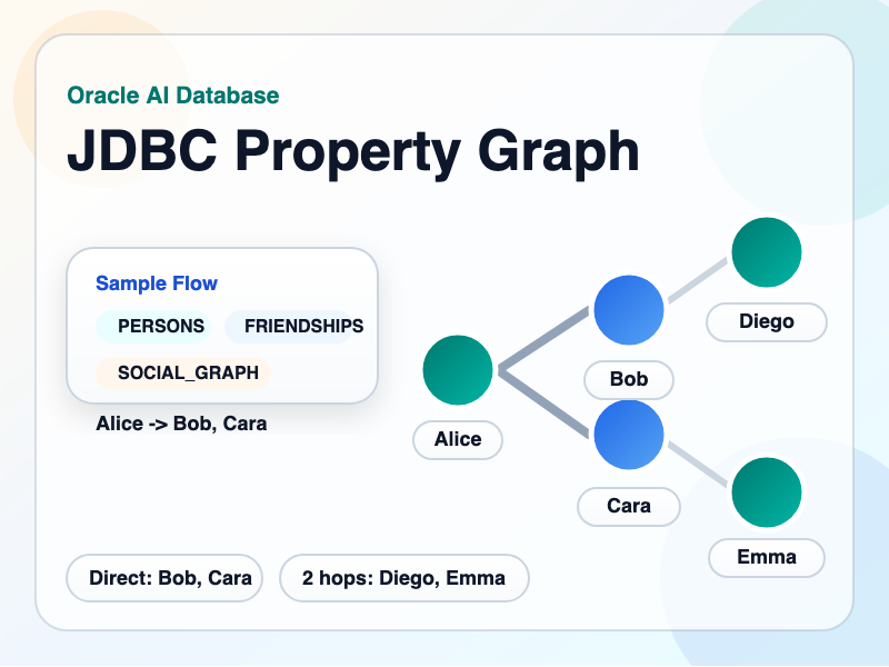
The sample models a small social graph:

• PERSONS is the vertex table
• FRIENDSHIPS is the edge table
• SOCIAL_GRAPH is the named property graph

From there, it demonstrates three graph queries:

• direct friends of a person
• everyone reachable within one or two hops
• recommended friends based on friends-of-friends

The data model is small, but the queries are interesting enough to show why graph syntax makes sense for specific types of relationships.

Why property graphs are useful

Most teams already store graph-shaped data in ordinary relational tables. However, it’s challenging to ask graph traversal questions to plain relational data:

• Who are Alice’s direct friends?
• Who is reachable from Alice in one or two hops?
• Which people are friends-of-friends, but not already direct friends?

Property graphs give you a simpler way to ask these questions. You get to keep your relational tables, adding a graph view designed for traversal. This graph view makes relationship-heavy queries much easier to read and reason about.

Sample relational schema

The sample begins with two relational tables, loaded with the resetSchema() method:

create table PERSONS (
    person_id number primary key,
    name varchar2(50) not null unique,
    hometown varchar2(50) not null
);
create table FRIENDSHIPS (
    friendship_id number primary key,
    person1_id number not null references PERSONS(person_id),
    person2_id number not null references PERSONS(person_id),
    since_year number(4) not null,
    strength number(3) not null,
    constraint friendship_not_self check (person1_id <> person2_id)
);

create table PERSONS (
    person_id number primary key,
    name varchar2(50) not null unique,
    hometown varchar2(50) not null
);
create table FRIENDSHIPS (
    friendship_id number primary key,
    person1_id number not null references PERSONS(person_id),
    person2_id number not null references PERSONS(person_id),
    since_year number(4) not null,
    strength number(3) not null,
    constraint friendship_not_self check (person1_id <> person2_id)
);

We also create indexes on FRIENDSHIPS(person1_id, person2_id) and FRIENDSHIPS(person2_id, person1_id) to support our access pattern.

Sample data is loaded in the loadSampleData() method, adding five people and relationships in the FRIENDSHIPS table. The graphed relationships look like this:

Creating the property graph

In the createPropertyGraph() method, we create a property graph using the CREATE PROPERTY GRAPH statement, with PERSONS for vertices and FRIENDSHIPS for edges:

create property graph SOCIAL_GRAPH
vertex tables (
    PERSONS
        key (person_id)
        label person
        properties (person_id, name, hometown)
)
edge tables (
    FRIENDSHIPS
        key (friendship_id)
        source key (person1_id) references PERSONS(person_id)
        destination key (person2_id) references PERSONS(person_id)
        label friend
        properties (friendship_id, person1_id, person2_id, since_year, strength)
)

create property graph SOCIAL_GRAPH
vertex tables (
    PERSONS
        key (person_id)
        label person
        properties (person_id, name, hometown)
)
edge tables (
    FRIENDSHIPS
        key (friendship_id)
        source key (person1_id) references PERSONS(person_id)
        destination key (person2_id) references PERSONS(person_id)
        label friend
        properties (friendship_id, person1_id, person2_id, since_year, strength)
)

This transforms the relational tables from plain relational data into a graph that can be traversed with graph algorithms.  “two relational tables” into “a graph I can traverse with graph patterns.”

Let’s break down the mapping:

• each row in PERSONS becomes a person vertex
• each row in FRIENDSHIPS becomes a friend edge
• vertex and edge properties stay available to the graph query layer

This makes your graph an abstraction over the relational data you already manage!

Querying the graph with GRAPH_TABLE

The sample exposes three small query methods:

• listDirectFriends(String personName)
• listFriendsWithinTwoHops(String personName)
• listRecommendedFriends(String personName)

Each one uses a GRAPH_TABLE query and returns a list of names. Let’s break them down, one-by-one.

One hop: direct friends

The first query starts with one person vertex and follows one outgoing friend edge:

select friend_name
from graph_table (SOCIAL_GRAPH
    match
    (start_person is person where start_person.name = ?)
        -[e is friend]->
    (friend is person)
    columns (friend.name as friend_name)
)
order by friend_name

select friend_name
from graph_table (SOCIAL_GRAPH
    match
    (start_person is person where start_person.name = ?)
        -[e is friend]->
    (friend is person)
    columns (friend.name as friend_name)
)
order by friend_name

If you call it with Alice, the sample returns:

[Bob, Cara]

[Bob, Cara]

One OR two hops: friends and friends-of-friends

The next query uses a path quantifier:

select distinct candidate_name
from graph_table (SOCIAL_GRAPH
    match
    (start_person is person where start_person.name = ?)
        -[e is friend]->{1,2}
    (candidate is person)
    where start_person.person_id <> candidate.person_id
    columns (candidate.name as candidate_name)
)
order by candidate_name

select distinct candidate_name
from graph_table (SOCIAL_GRAPH
    match
    (start_person is person where start_person.name = ?)
        -[e is friend]->{1,2}
    (candidate is person)
    where start_person.person_id <> candidate.person_id
    columns (candidate.name as candidate_name)
)
order by candidate_name

-[e is friend]->{1,2}, means “follow this edge one or two times.” For Alice, this query includes both direct friends and friends-of-friends:

[Bob, Cara, Diego, Emma]

[Bob, Cara, Diego, Emma]

Indirect: recommended friends

The last query finds two-hop candidates, and removes anyone who is already a direct friend, groups the results, and sorts by the number of common-friend paths:

select candidate_name
from (
    select candidate_name, count(*) as common_friend_count
    from graph_table (%s
        match
        (person is person where person.name = ?)
            -[first_hop is friend]->
        (common_friend is person)
            -[second_hop is friend]->
        (candidate is person)
        where person.person_id <> candidate.person_id
        columns (candidate.name as candidate_name)
    )
    where candidate_name not in (
        select friend_name
        from graph_table (%s
            match
            (person is person where person.name = ?)
                -[direct_edge is friend]->
            (friend is person)
            columns (friend.name as friend_name)
        )
    )
    group by candidate_name
)
order by common_friend_count desc, candidate_name

select candidate_name
from (
    select candidate_name, count(*) as common_friend_count
    from graph_table (%s
        match
        (person is person where person.name = ?)
            -[first_hop is friend]->
        (common_friend is person)
            -[second_hop is friend]->
        (candidate is person)
        where person.person_id <> candidate.person_id
        columns (candidate.name as candidate_name)
    )
    where candidate_name not in (
        select friend_name
        from graph_table (%s
            match
            (person is person where person.name = ?)
                -[direct_edge is friend]->
            (friend is person)
            columns (friend.name as friend_name)
        )
    )
    group by candidate_name
)
order by common_friend_count desc, candidate_name

For Alice, the sample returns:

[Emma, Diego]

[Emma, Diego]

These property graph queries are still SQL, but use graph traversal logic instead of join chains.

The Java side

One of the best things about this module is that the Java code stays very plain, making the query logic portable to other languages. The sample main method takes three arguments:

• JDBC URL
• username
• password

From there it:

1. builds a pooled datasource
2. recreates the schema
3. loads the sample data
4. creates the property graph
5. runs the graph queries
6. writes the SVG output

No separate graph service, no special client stack, and no framework to using graph features working. Just plain JDBC and SQL.

Run it locally

If you want to test the sample (JdbcPropertyGraphSampleTest.java) end to end with Testcontainers, run:

mvn test

mvn test

It starts Oracle AI Database Free, grants CREATE PROPERTY GRAPH to the test user, runs the sample, and checks the query results.

If you want to run the application directly against your own database user, make sure that user has the required privilege:

grant create property graph to your_user;

grant create property graph to your_user;

Then run:

mvn exec:java -Dexec.args="jdbc:oracle:thin:@localhost:1521/freepdb1 testuser testpwd"

mvn exec:java -Dexec.args="jdbc:oracle:thin:@localhost:1521/freepdb1 testuser testpwd"

You should see output similar to:

Direct friends of Alice: [Bob, Cara]
Friends within two hops of Alice: [Bob, Cara, Diego, Emma]
Recommended friends for Alice: [Emma, Diego]
Property graph diagram written to: ./jdbc-property-graph/property-graph-diagram.svg

Direct friends of Alice: [Bob, Cara]
Friends within two hops of Alice: [Bob, Cara, Diego, Emma]
Recommended friends for Alice: [Emma, Diego]
Property graph diagram written to: ./jdbc-property-graph/property-graph-diagram.svg

Next steps

If you want a small example you can actually run, inspect, and extend, this module is a solid place to start:

• jdbc-property-graph source code
• You can also refer to the property graph documentation